
Introduction
Lately, I’ve found myself bewitched by Bayesian modeling—even to the point of reading textbooks(!!) in my off-hours, to my wife’s dismay. I’ve had a passing familiarity with Bayesian methods in the past, though mostly through casual reading about the latest and greatest models in fields like bioinformatics and neuroscience, where it’s well-established and more mature. Nothing more concrete than that, really. When I covered Bayes’ Theorem in a previous post, I grasped the theorem itself and the basics of how to use it in out-of-the-box models like Naïve Bayes, but I never fully understood how Bayesian inference could practically fit into my everyday data science work.
Early this year, however, my curiosity deepened and I began to read into comparisons between Bayesian methods and their much more ubiquitous frequentist counterparts (see table below for a brief explanation). Coincidentally, just a few months ago, I had the perfect opportunity for applying Bayesian methods fall into my lap, with resounding success. That experience highlighted for me the immense advantages Bayesian inference offers—particularly its interpretability, intuitive nature, and strength in handling small sample sizes.
Frequentist vs Bayesian: Quick Comparison
| Frequentists | Bayesians | |
|---|---|---|
| Hypothesis testing | Set null and alternative hypotheses and use statistical tests to assess evidence against the null. | Consider prior beliefs when forming hypotheses. |
| Probability interpretation | Frame probability in terms of objective, long-term frequencies. | Interpret probabilities subjectively and update them as new data is collected. |
| Sampling | Emphasize random sampling and often require fixed sample sizes. | Can adapt well to varying sample sizes since Bayesians update their beliefs as more data comes in. |
Table credit: Amplitude
Why Bayesian? A Real-World Motivation
At the heart of Bayesian methods is this defining feature: the integration of prior knowledge directly into the modeling process. Amazingly to me, this prior knowledge doesn’t necessarily have to come in the form of hard data. Instead, Bayesian modeling can natively incorporate various types of prior knowledge, such as:
- Your personal beliefs or expectations
- Expert opinions
- Domain-specific insights
- Historical or previously collected data
This flexibility fundamentally distinguishes Bayesian modeling from the statistical toolbox I’d used virtually exclusively up until recently—the very same that most statisticians, researchers, and analysts are familiar with. This feature makes Bayesian modeling not only powerful but uniquely intuitive. Below, I’ve put together a very digestible scenario and simulated data to demonstrate, in a piecemeal fashion, what this means for making inferences from your data.
Example Scenario
Imagine you work for a medical device company developing a new wearable sensor for health metrics such as blood glucose or blood pressure. Getting approval for a new medical device requires careful monitoring, and early-stage devices usually involve small samples sizes and some unexpected measurement error that requires calibration to some ground-truth data. In the following walkthrough, I’ll demonstrate how different statistical approaches handle these challenges and particularly how Bayesian modeling offers remarkable flexibility in incorporating prior knowledge and making your inferences robust to outlier data.
The Role of Prior Knowledge: Slope Expectation
Before we dive into the data, let’s call out a key piece of prior knowledge that will shape our Bayesian approach. In engineering and device calibration, domain experts often expect the relationship between reference and device measurements (when scaled appropriately) to be nearly linear, with a slope close to 1. This expectation is grounded in both physics and years of experience with similar devices. In Bayesian modeling, we can encode this expert opinion directly as a prior on the slope parameter. We’re telling the model, “We strongly believe the slope should be near 1, but we’re open to being convinced otherwise by the data.”
This is a major advantage over frequentist approaches, which have no natural way to formally incorporate such expert beliefs. In a frequentist regression, all parameters are estimated solely from the observed data, and there’s no mechanism to nudge the model toward what we already know from engineering or prior studies.
In the analysis below, you’ll see how this strong prior on the slope is incorporated into the Bayesian models, and how it helps the model remain robust even in the presence of outliers or small sample sizes.
Simulating Calibration Data
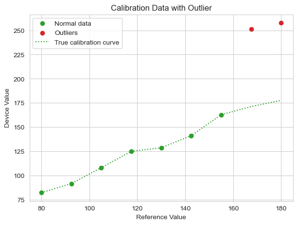
We begin by simulating a dataset mirroring a common real-world scenario, a new batch of devices is calibrated against some gold-standard reference. For example, you could be comparing a small batch of wearable glucose monitors against a real-time continuous glucose monitor in a clinical setting. Regardless of the details, in this example most of the devices perform as expected, but two of the devices malfunction or are flawed, generating outlier data points.
Importantly, past data with similar devices suggests that we suspect that the slope of this relationship should be near 1, with some variance, and that we don’t have very strong beliefs about the intercept. This means that we know that reference values should scale linearly with the device-measured values, but we’re not sure how much we’ll have to correct for—a very reasonable scenario!
import numpy as np
import pandas as pd
import matplotlib.pyplot as plt
import seaborn as sns

sns.set_style("whitegrid")

# Simulate 'true' calibration: y = x + noise
np.random.seed(42)
n = 9
x = np.linspace(80, 180, n)
noise = np.random.normal(0, 5, n)  # Small gaussian noise
y_true = x + noise

# Add severe outlier
y = y_true.copy()
y[-1] = y_true[-1] + 80  # Last data point is an outlier
y[-2] = y_true[-2] + 80  # Second to last data point is also an outlier
Plotting the data, we see a clear linear trend except for two high outliers at the right end of the scatterplot. Alongside the data points is the true calibration curve for the “good” data points. If we were constructing a calibration model, this curve made by the observed data would be used to provide an offset to correct for error between the wearable device and the baseline measurement.
# Plotting the good data points, outliers, and the true calibration curve
plt.figure(figsize=(7, 5))
plt.scatter(
    x[:-2],
    y[:-2],
    color="C2",
    label="Normal data",
)
plt.scatter(
    x[-2:],
    y[-2:],
    color="C3",
    label="Outliers",
)
plt.plot(
    x,
    y_true,
    color="C2",
    linestyle=":",
    label="True calibration curve",
)
plt.xlabel("Reference Value")
plt.ylabel("Device Value")
plt.title("Calibration Data with Outlier")
plt.legend()
plt.show()
The natural inclination for many analysts or researchers would be to fit a linear regression (ordinary least squares, or OLS) to the observed data. We’ll do that below.
Frequentist Modeling Approaches
OLS Regression
An OLS regression, the straight-line, fit-a-line-to-the-data regression model that everyone knows, tries to minimize the sum of squared errors across all data points. This method treats every data point as valid and equally weighted.
# Helper function to plot points
def plot_points():
    plt.scatter(
        x[:-2],
        y[:-2],
        color="C2",
        label="Data points",
    )
    plt.scatter(
        x[-2:],
        y[-2:],
        color="C3",
        label="Outliers",
    )
import statsmodels.api as sm

X = sm.add_constant(x)  # Add constant for intercept
ols_model = sm.OLS(y, X)  # OLS regression model
ols_result = ols_model.fit()
print(ols_result.summary())

# Plot OLS regression line over the data
plt.figure(figsize=(7, 5))
plot_points()
plt.plot(
    x,
    ols_result.fittedvalues,
    color="C0",
    label="OLS Regression Line",
)
plt.xlabel("Reference Value")
plt.ylabel("Device Value")
plt.title("Frequentist OLS Regression")
plt.legend()
plt.show()
                            OLS Regression Results
==============================================================================
Dep. Variable:                      y   R-squared:                       0.864
Model:                            OLS   Adj. R-squared:                  0.844
Method:                 Least Squares   F-statistic:                     44.32
Date:                Tue, 24 Jun 2025   Prob (F-statistic):           0.000289
Time:                        14:23:59   Log-Likelihood:                -40.717
No. Observations:                   9   AIC:                             85.43
Df Residuals:                       7   BIC:                             85.83
Df Model:                           1
Covariance Type:            nonrobust
==============================================================================
                 coef    std err          t      P>|t|      [0.025      0.975]
------------------------------------------------------------------------------
const        -76.1982     35.003     -2.177      0.066    -158.966       6.570
x1             1.7397      0.261      6.658      0.000       1.122       2.358
==============================================================================
Omnibus:                        0.808   Durbin-Watson:                   1.183
Prob(Omnibus):                  0.668   Jarque-Bera (JB):                0.564
Skew:                          -0.022   Prob(JB):                        0.754
Kurtosis:                       1.775   Cond. No.                         556.
==============================================================================

Notes:
[1] Standard Errors assume that the covariance matrix of the errors is correctly specified.
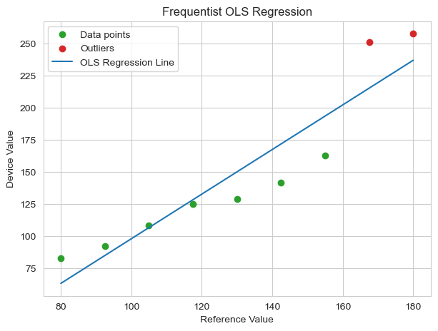
The resulting regression line is very obviously pulled upward by the two outlier data points. As a result, our OLS model is simultaneously underpredicting the low reference value data points and overpredicting the high reference value data points. In other words, the outliers are distorting the calibration, making the model less accurate for the majority of the well-behaved data.
Ridge Regression
A way that a modeler might combat the effect of outliers in regression would be to employ regularization—a method for reducing model overfitting by penalizing large coefficient values. This approach encourages simpler models that generalize better, making them less sensitive to outliers. Below, we implement Ridge regression, which applies an L2 penalty (the sum of squared coefficients) to the loss function. This penalty discourages the model from assigning excessive weights to any single feature, enhancing robustness against the two outliers. Due to the small sample size, we’re using a large alpha value (1000).
# Ridge regression using statsmodels' WLS with a penalty matrix
alpha = 1000  # Ridge penalty
penalty = np.diag([0, alpha])
XTX = np.dot(X.T, X) + penalty
XTy = np.dot(X.T, y)
ridge_coef = np.linalg.solve(XTX, XTy)

print("Ridge regression coefficients (intercept, slope):", ridge_coef)

# Predicted values
y_ridge = np.dot(X, ridge_coef)

plot_points()
# Plot OLS and Ridge regression lines
plt.plot(
    x,
    ols_result.fittedvalues,
    color="C0",
    label="OLS Regression Line",
)
plt.plot(x, y_ridge, color="C1", label="Ridge Regression Line")
plt.xlabel("Reference Value")
plt.ylabel("Device Value")
plt.title(f"Frequentist OLS vs Ridge Regression")
plt.legend()
plt.show()
Ridge regression coefficients (intercept, slope): [-54.39929082 1.5720375 ]
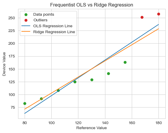
While showing a small improvement in the model fit to the good data, with only nine data points, two outliers constitute approximately 22% of the dataset. Ridge regression’s penalty becomes less effective when outliers have such high leverage. The regularization strength would need to be so high that it would severely bias the slope away from the true value of 1. This calibration is far from optimal.
At this junction, Bayesian modeling offers a major leap in adaptability. While with frequentist methods, unless we alter the dataset, we must work with the data that we have (despite its flaws), with a Bayesian framework we can explicitly encode our knowledge and expectations into the model: The device should have a slope near 1 (matching the reference data).
Bayesian Modeling Framework
In the Bayesian models below, we explicitly encode our strong prior belief: based on expert opinion and engineering knowledge, the slope should be near 1. This is a key difference from the frequentist models above.
Bayesian Regression with Informed Priors
In the model below, we’re defining the same basic linear model as with the frequentist models: y = mx + b. However, because Bayesian models estimate the posterior distributions rather than point estimates, they provide a richer understanding of the uncertainty surrounding the model parameters. Instead of producing a single “best-fit” line, Bayesian regression generates a distribution of plausible lines based on the prior knowledge and observed data. This allows us to incorporate domain-specific expectations (e.g., the slope should be near 1) directly into the modeling process, making the model more robust to outliers and small sample sizes. By leveraging informed priors, we can guide the model toward solutions that align with our prior beliefs about the relationship while still allowing the data to refine those beliefs. This flexibility is a key advantage of Bayesian methods over traditional frequentist approaches, especially at small sample sizes.
In the model below, we use wide, uninformative prior distributions for the intercept and noise—we don’t have strong beliefs about what those parameters look like. However, we do implement a strong, informative prior on the slope (see the narrow sigma value: 0.1 vs. 50). We know from past data and expert knowledge that the slope should be near 1, so we encode this as a Normal distribution centered at 1, with a variance of 0.1. ~95% of estimated slope values will fall between 0.8 and 1.2. We also use a normal likelihood, which states that the observed data points are normally distributed around the true regression line, which is a typical assumption of linear regression.
import pymc as pm
import arviz as az

with pm.Model() as bayesian_model:
    # Strong prior: slope ~= 1
    intercept = pm.Normal("intercept", mu=0, sigma=50)
    slope = pm.Normal("slope", mu=1, sigma=0.1)
    sigma = pm.HalfNormal("sigma", sigma=50)
    mu = intercept + slope * x  # Linear model
    y_obs = pm.Normal("y_obs", mu=mu, sigma=sigma, observed=y)
    trace = pm.sample(
        1000,
        tune=1000,
        nuts_sampler="numpyro",
        return_inferencedata=True,
        random_seed=42,
        progressbar=False,
    )

print(az.summary(trace, hdi_prob=0.95).to_string())
az.plot_trace(
    trace,
    var_names=["intercept", "slope", "sigma"],
    combined=True,
    figsize=(7, 5),
)
plt.tight_layout()
plt.show()
             mean      sd  hdi_2.5%  hdi_97.5%  mcse_mean  mcse_sd  ess_bulk  ess_tail  r_hat
intercept  11.935  17.284   -20.818     46.787      0.404    0.296    1825.0    2029.0    1.0
slope       1.058   0.097     0.867      1.240      0.002    0.002    1963.0    2691.0    1.0
sigma      37.262   9.916    20.333     56.085      0.205    0.248    2404.0    2400.0    1.0
# Bayesian posterior predictive mean
slope_mean = trace.posterior["slope"].mean().item()
intercept_mean = trace.posterior["intercept"].mean().item()
# Predictions
y_bayesian = intercept_mean + slope_mean * x

# Plot showing Ridge and Bayesian regression lines
plot_points()
plt.plot(x, y_ridge, color="C1", label=f"Ridge Regression Line")
plt.plot(
    x,
    y_bayesian,
    color="C4",
    label="Bayesian Regression Line",
)
plt.xlabel("Reference Value")
plt.ylabel("Device Value")
plt.title("Frequentist Ridge vs Bayesian Regression")
plt.legend()
plt.show()
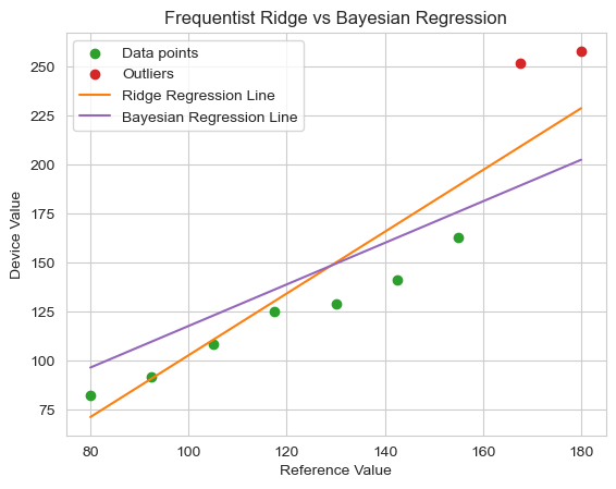
The Bayesian model, with guidance from the prior knowledge, estimates the approximate slope that we anticipated (1.058). Visually, we can see a major improvement, yet we intentionally didn’t encode any beliefs about the intercept within the model (because there are many reasons we wouldn’t have good prior knowledge of a parameter) and the outliers are pulling the intercept estimate upward. The model is trying to satisfy both the prior (slope ~= 1) and the data. So, we’ve got this lingering effect of the outliers causing our model to overpredict at every good data point. How can we resolve this?
Well, one of the things I like very much about Bayesian modeling is that it forces you to confront your assumptions when developing a model. Standard linear regression (OLS) assumes that the data will be distributed normally about the regression line (i.e. normally distributed residuals). That is definitely not the case here, as all of the good data points reside below our prediction. The Normal likelihood assumption is sensitive to outliers. With a Bayesian framework, we can ditch this assumption and use the distribution of our choice in the likelihood function we define.
Bayesian Regression with Student’s T Likelihood
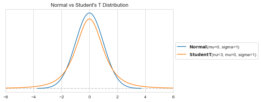
A great option for our likelihood problem is the Student’s T distribution. While at first glance very similar to the Normal distribution, the Student’s T distribution has heavier tails. This characteristic makes it more robust to outliers, as it assigns higher probabilities to extreme values compared to the Normal distribution. By using the Student’s T distribution as our likelihood function for the observed data, we can mitigate the influence of outliers on the parameter estimates, resulting in a more accurate and reliable model!
import preliz as pz

# Define distributions
plt.figure(figsize=(7, 3.5))
normal_dist = pz.Normal(mu=0, sigma=1).plot_pdf()
student_t_dist = pz.StudentT(mu=0, sigma=1, nu=3).plot_pdf()
plt.xlim(-6, 6)
plt.title("Normal vs Student's T Distribution")
plt.show()
It only requires a minor tweak to the model:
with pm.Model() as bayesian_model_student_t:
    # Strong prior: slope ~= 1
    intercept = pm.Normal("intercept", mu=0, sigma=10)
    slope = pm.Normal("slope", mu=1, sigma=0.1)
    sigma = pm.HalfNormal("sigma", sigma=10)
    mu = intercept + slope * x  # Linear model
    y_obs = pm.StudentT(
        "y_obs", mu=mu, sigma=sigma, nu=3, observed=y
    )  # Student's t-distribution for robustness
    trace_student_t = pm.sample(
        1000,
        tune=1000,
        nuts_sampler="numpyro",
        return_inferencedata=True,
        random_seed=42,
        progressbar=False,
    )

print(az.summary(trace_student_t, hdi_prob=0.95).to_string())
             mean     sd  hdi_2.5%  hdi_97.5%  mcse_mean  mcse_sd  ess_bulk  ess_tail  r_hat
intercept  -2.264  8.337   -18.187     14.387      0.210    0.157    1582.0    1824.0    1.0
slope       1.066  0.079     0.920      1.228      0.002    0.002    1481.0    1537.0    1.0
sigma      12.194  4.640     4.159     21.575      0.132    0.069    1092.0     930.0    1.0
# Bayesian posterior predictive mean
slope_mean_student_t = trace_student_t.posterior["slope"].mean().item()
intercept_mean_student_t = trace_student_t.posterior["intercept"].mean().item()
# Predictions
y_bayesian_student_t = intercept_mean_student_t + slope_mean_student_t * x

plot_points()
plt.plot(
    x,
    y_bayesian,
    color="C4",
    label="Bayesian Regression Line (Normal Likelihood)",
)
plt.plot(
    x,
    y_bayesian_student_t,
    color="C6",
    label="Bayesian Regression Line (Student-T Likelihood",
)
plt.xlabel("Reference Value")
plt.ylabel("Device Value")
plt.title("Comparison of Regression Models")
plt.legend()
plt.show()
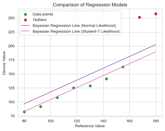
This change yields a considerable final improvement in our model. The regression line now hugs the well-behaved device data, nearly ignoring the outliers completely.* The model fit is both statistically robust and faithful to the prior knowledge we had about the relationship between device and reference measurements.
* You might say, just drop the outliers, problem solved. But for the the following reasons, this is not usually recommended (especially in healthcare/medical domains):
- It is subjective and risky
- Your models should reflect reality and be transparent
- Regulatory and scientific rigor requirements demand that you don’t
- Flexibility for future data—a robust model will automatically adjust
Conclusion
Though revealed via a toy example, this sequence of modeling choices demonstrates the unique flexibility of Bayesian modeling. Not only can we formally incorporate unstructured prior knowledge through informative priors, but we can also tailor the model to handle specific characteristics of the problem, such as the presence of outliers, without compromising the integrity of the inference process. Where frequentist methods are sometimes limited by rigid assumptions, the Bayesian framework allows us to build models that reflect both what we know and what the data reveals, leading to more robust and interpretable results.
In the next post, I plan to explore another key feature of Bayesian modeling: its ability to produce full probability distributions instead of single point estimates, offering deeper insight into uncertainty and variability.
Bonus: From Point Estimates to Probabilistic Insights
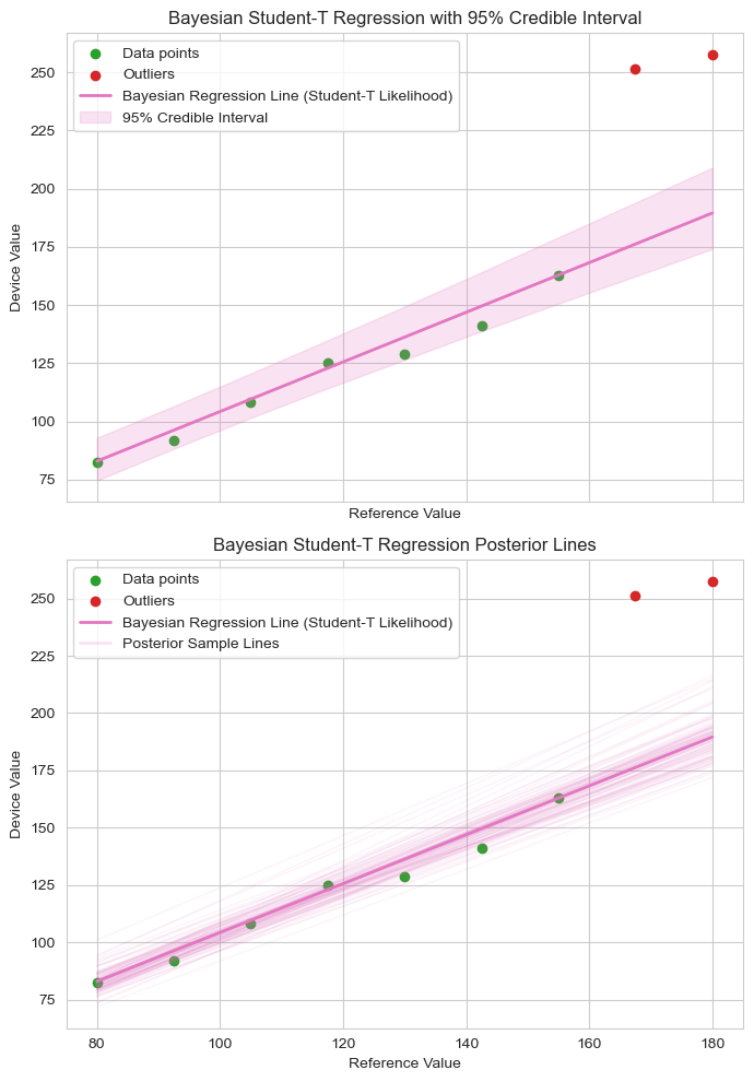
Unlike traditional regression models that yield a single best-fit line, because Bayesian inference outputs probability distributions rather than single point-estimates, Bayesian regression provides a far richer insight of the model and its parameters. This means we don’t just estimate the most likely slope or intercept—we also quantify our uncertainty about them. The result is a distribution of plausible regression lines, each consistent with the observed data and our prior beliefs. The first plot below illustrates this with a shaded 95% credible interval (the area that the 95% most likely fits fall into) around the mean regression line, while the second plot reveals the deeper story: 100 regression lines sampled from the posterior, showing the range of plausible relationships supported by the model.
from matplotlib.lines import Line2D

# Compute 95% credible interval for predictions from the Student-T model
posterior = trace_student_t.posterior
slope_samples = posterior["slope"].values.flatten()
intercept_samples = posterior["intercept"].values.flatten()

# Vectorized computation of predicted y for all posterior samples
y_pred_samples = intercept_samples[:, None] + slope_samples[:, None] * x

# Compute 2.5 and 97.5 percentiles for each x
y_lower, y_upper = np.percentile(y_pred_samples, [2.5, 97.5], axis=0)

fig, axes = plt.subplots(2, 1, figsize=(7, 10), sharex=True)

# First plot: regression line with 95% credible interval
ax = axes[0]
plt.sca(ax)
plot_points()
ax.plot(
    x,
    y_bayesian_student_t,
    color="C6",
    label="Bayesian Regression Line (Student-T Likelihood)",
    linewidth=2,
)
ax.fill_between(
    x,
    y_lower,
    y_upper,
    color="C6",
    alpha=0.2,
    label="95% Credible Interval",
)
ax.set_xlabel("Reference Value")
ax.set_ylabel("Device Value")
ax.set_title("Bayesian Student-T Regression with 95% Credible Interval")
ax.legend()

# Second plot: regression line with posterior sample lines
ax = axes[1]
plt.sca(ax)
plot_points()
num_lines = 100
idx = np.random.choice(y_pred_samples.shape[0], num_lines, replace=False)
for i in idx:
    ax.plot(x, y_pred_samples[i], color="C6", alpha=0.08, linewidth=1)
ax.plot(
    x,
    y_bayesian_student_t,
    color="C6",
    label="Bayesian Regression Line (Student-T Likelihood)",
    linewidth=2,
)
# Legend wrangling
posterior_proxy = Line2D(
    [0], [0], color="C6", alpha=0.2, linewidth=2, label="Posterior Sample Lines"
)
handles, labels = ax.get_legend_handles_labels()
handles.append(posterior_proxy)
labels.append("Posterior Sample Lines")
ax.set_xlabel("Reference Value")
ax.set_ylabel("Device Value")
ax.set_title("Bayesian Student-T Regression Posterior Lines")
ax.legend(handles, labels)

plt.tight_layout()
plt.show()
Stay tuned for more!
- Jacob