Update October 2024
I have been very, very busy between work, finishing my master’s degree, and home life. I intended for this “Demystifying Algorithms” series to continue (particularly with a follow-up piece on Naïve Bayes classifiers), but alas, it’s DOA. I’ll have plenty to share in the future, but other priorities have obviously taken precedence!
Get the Fundamentals Down
Short-Term Plan
As I touched on in my previous post discussing the differences between AI and machine learning, we’ve recently seen a surge in the complexity and pervasiveness of large language models (LLMs) like OpenAI’s ChatGPT and Google’s Bard. While these deep learning models deservedly receive much of the spotlight of public attention as a result of their complexity and their ability to create human-like text on demand, I believe it is important to recognize some of the underlying elements and algorithms that make these state of the art models possible.
I think what I would like to do, at least for a few posts (who knows, maybe more!), is to introduce some foundational algorithms and models in machine learning, many of which form the underpinnings of the more advanced, popular AI models. I’d like to cover why they are important and relevant, their common use-cases, and I’d like to step through their inner-workings in relatively plain language.
Bayesian Fusion
When you start to pick apart the world of machine learning and AI in general, it becomes clear that, similar to the fields of mathematics or chemistry, modern achievements are built upon the work of those that came before. We can’t begin to build predictive and generative models without first understanding foundational elements of probability. Because without estimating the probability of an event, how would you ever hope to predict it or generate outcomes based on it?
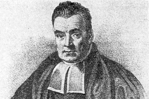
One of these foundational elements of machine learning, and what I’d like to delve into today, is Bayes’ Theorem and its derivative, the Naïve Bayes algorithm. These pieces of machine learning application help bridge the gap between mathematical theory and practical applications in AI. Originating from the work of its namesake, 18th-century mathematician, philosopher, and minister, Thomas Bayes, Bayes’ Theorem creates a framework for relating probabilities and estimating the change in probability of an event, given new observed evidence. [1] In essence, it allows you to update beliefs, in light of new information. It is a component under the hood of many of today’s machine learning-based tools. Common applications include email/text spam filtering, medical diagnostic systems, search engine recommendations, and more. Pivoting from the world of these and more advanced models, let’s dive into Bayes’ Theorem and Naïve Bayes models to illustrate how relatively simple concepts can be extended out into complex systems to empower and elevate artificial intelligence.

Understanding Bayes’ Theorem
A Palatable Example
Imagine that you are a person who, for some time, have heard and lived by the advice that all carbohydrates are detrimental to your health. You read a magazine that anyone concerned about their health should go out of their way to avoid carbs at all costs, be it crackers, cereals, bread, or sweets. After a while of eating nothing only fats and protein, you begin to feel lethargic and easily drained. You get headaches and can’t seem to think clearly. At the suggestion of a friend, you make an appointment with a nutritionist. During this consultation, this nutritionist tells you that actually, carbs aren’t such a bad thing. Sure, you should balance them with the other macronutrients and make sure you’re prioritizing slower-digesting starches over sucrose and fructose in sweets, but she tells you that your brain actually needs a minimal amount of carbohydrates to function properly! So what should you do?
This situation exemplifies a case where your beliefs are directly contradicted by new information. It is highly likely that revising your dietary opinions based on a licensed nutritionist’s recommendation, rather than what a sensationalized magazine article suggests, would be more beneficial. To make an informed decision about your diet, you need to update your belief system, taking into consideration this advice. This process of revising beliefs in the light of new, credible evidence is a practical application of Bayes’ Theorem, where prior beliefs are updated with new data to form a more accurate understanding or hypothesis.
Practical Application - Another Healthy Dose
So, we can think of a situation where one might have to change their beliefs due to specific circumstances, how is this actually applied in probability theory? Bayes’ Theorem can be a little difficult to wrap your brain around for new learners, but once you crack it, it becomes clear how elegant it actually is. I’ll ease you into it with another example.
Say that there is a rare disease, Boogie Fever that 2% of the human population carries a hereditary gene for. So, out of every one hundred people, two of them will develop Boogie Fever at some point in their lifetime. There is a test for this gene that is pretty good but isn’t perfect, like all medical tests. It correctly identifies people with the Boogie Fever gene 95% of the time for people who actually have it (sensitivity of 95%), and it will correctly show a negative result 90% of the time for people who don’t have it (specificity of 90%). Let’s show the information we know so far:
Gene Prevalence (Prior Probability): 2%. We know that on average, 2 in 100 people actually have the gene for Boogie Fever.
Test Sensitivity (True Positive Rate): 95%. The test will correctly identify the Boogie Fever gene in 95% of those who have it.
Test Specificity (True Negative Rate): 90%. The test will correctly show a negative result for 90% of people who don’t carry the gene.
 Shoutout to DALL-E for letting me get this creative.
Now, suppose that Bob walks into the Midnight Special’s Center for Boogie Fever Research and gets tested. Bob gets a positive result in the mail two weeks later, telling him that he’s likely to carry the Boogie Fever gene. But just how likely? What is the probability that Bob carries the gene, given his positive test result?
This is where Bayes’ Theorem allows us to do some probabilistic magic. Here is the formula:
\[P(A|B) = \frac{P(B|A) \cdot P(A)}{P(B)}\]This formula should give you an idea of the kind of conditional probability inferences that we can make using the concept represented by Bayes’ Theorem. British geophysicist and significant contributor to the field of probability theory, Sir Harold Jeffreys, described the theorem as “to the theory of probability what Pythagoras’s theorem is to geometry”.[2] Just as the Pythagorean Theorem is used to infer previously unknown relationships in geometry, Bayes’ Theorem lets you infer new probabilities using relationships.
“[Bayes’ Theorem] is to the theory of probability what the Pythagorean theorem is to geometry.”
Sir Harold Jeffreys
Given the information we have about Bob’s situation, we can apply the theorem with a little added complexity. This additional complexity is due to the fact that we’re not just interested in the direct relationship between having the Boogie Fever gene and testing positive. Instead, we want to know the probability of having the gene, given a positive test result. This is a more complex scenario because we have to consider two possibilities for a positive test result, a true positive and false positive. I won’t go into depth on the additions for accounting for false results, but this is the extended generic equation:
\[P(A|B) = \frac{P(B|A) \cdot P(A)}{P(B|A) \cdot P(A) + P(B|\neg A) \cdot P(\neg A)}\]This new equation, taking into account the accuracy of the test, prevalence of the gene, and two cases for positive and negative results respectively, provides a more accurate assessment of the likelihood of having the gene in the context of real-world testing scenarios. Plugging our scenario in looks like this:
\[P(\text{Gene} | \text{Positive Test}) = \frac{P(\text{Positive Test} | \text{Gene}) \cdot P(\text{Gene})}{P(\text{Positive Test} | \text{Gene}) \cdot P(\text{Gene}) + P(\text{Positive Test} | \text{No Gene}) \cdot P(\text{No Gene})}\]And thus, adding in our probabilities provides us with the answer:
\[P(\text{Gene} | \text{Positive Test}) = \frac{ 0.95 \cdot 0.02 }{ 0.95 \cdot 0.02 + 0.10 \cdot 0.98} \approx 0.16239\]Bob might receive his test result and be struck by the thought that he’s doomed to develop Boogie Fever. But with a little probability inference, we have calculated that despite his positive result, there’s only a roughly 16% chance that he actually carries the gene! So, not everything is as clear cut as it initially seems. This example illustrates just a single circumstance where Bayes’ theorem is useful in estimating a conditional probability from related probabilities. It also underscores the balancing act between sensitivity and specificity in medical diagnostic testing design. It’s very important that the test is sensitive in that it detects what you’re looking for, but it’s maybe equally important to limit the amount of false positives that come with a low specificity.
But, we’re not done just yet. Let’s prove this estimate with some simulation!
Simulating Probabilities
Using Python, I will demonstrate the above scenario by simulating testing patients using randomly generated numbers. I won’t step through every line of the code, but in essence, it simulates 1 million patients with a gene prevalence of 2%, a test sensitivity of 95% (true positive rate), and specificity of 90% (true negative rate). Note that due to the stochastic nature of this simulation, it will result in a final probability that might differ slightly from our estimated probability of ~16.24%. However, it ought to be very close, as Bayes’ Theorem gave us the mathematical framework to properly estimate it. The code follows:
# Importing numpy
import numpy as np

# Parameters for the scenario
population = 1000000 # size of the population to simulate
prevalence = 0.02 # 2% of the population has the gene
sensitivity = 0.95 # true positive rate
specificity = 0.90 # true negative rate

# Simulating the population
# True for individuals with the gene, False for those without
gene = np.random.rand(population) < prevalence

# Simulating test results
# True for a positive test, False for a negative test
positive_test_given_gene = np.random.rand(population) < sensitivity
negative_test_given_no_gene = np.random.rand(population) < specificity

# True positive: gene and positive test
# False positive: no gene but positive test
positive_test = (gene & positive_test_given_gene) | (~gene & ~negative_test_given_no_gene)

# Calculating the probability of having the gene given a positive test result and outputting
probability_gene_given_positive_test = np.mean(gene[positive_test])
print(probability_gene_given_positive_test)0.16203537554473213As we can see from the output above, the simulated probability of having the Boogie Fever gene given a positive test result is ~16.2%. Aside from a discrepancy of a few hundredths of a percentage point, we are spot on! It’s clear that this is a highly performant way to update probability estimates in light of new evidence.
Moving from Theorem to Model
The practical implications of Bayes’ Theorem, seen in this example various real-world applications, underline its significance in increasingly complex and sophisticated AI models. The theorem considerably underpins the field of probability theory and it is built upon even further as we move from relatively simple probabilistic calculations to building complex predictive models. While I have yet to delve into the Naïve Bayes models, this initial discussion sets the stage for a deeper exploration in Part II! Through the process of writing this piece, I decided to break this up into two parts in order to truly dedicate enough of my discussion to the base theory before delving into the predictive power it provides under the hood of models such as Naïve Bayes. In the next post, I’ll cover how these models can lend predictive power to detecting the tone and sentiment of book reviews!
Stay tuned,
- Jacob
References
- Wikipedia: Bayes’ Theorem
- Jeffreys, Harold (1973). Scientific Inference (3rd ed.). Cambridge University Press. p. 31

